Inspections in Customs: A Case Study of the Role of Tariff Dispersion on Red Lane Classification in Argentina

1. Introduction

In international trade, Customs represent the doorkeepers of each country (Martincus et al., 2013). They play a key role at every border, preventing the entrance of illegal products and dangerous or hazardous materials, and guaranteeing the safety and quality of products through, for example, technical barriers to trade (TBTs) or sanitary and phytosanitary measures (PSMs). Customs also represents, in many cases, the primary source of tax revenues (Morini et al., 2017).

However, Customs can also generate unnecessary delays, harming exports and trade (Martincus et al., 2013), competitiveness (Hoffman et al., 2021), or countries’ efficiency and responses to disasters (Turner, 2015). Therefore, reducing time delays in customs clearance becomes an important goal for every customs administration. In addition, the high levels of administrative bureaucracy, the low probability of being caught, and the extensive number of situations in which discretional decisions must be made make Customs a natural place for corruption, regardless of economic growth (Chalendard et al., 2021; McLinden & Durrani, 2013; Sequeira & Djankov, 2010; Stasavage & Daubrée, 1998).

Here, we focus on a new factor that might contribute to delays in Customs: import tariff dispersion. Tariff dispersion is defined as the ‘inequality of the tariffs levied by a country’ (Deardorff, n.d.), and it is usually measured in any import tariff structure by taking the standard deviation of tariff rates (Cooper, 1964; World Bank, n.d.). In the extreme case, if every product has the same import tariff (a flat import structure tariff, like the one Chile applies, or the countries of the Gulf Cooperation Council, such as the United Arab Emirates or Saudi Arabia), then the tariff dispersion would be zero.

In this paper, we analysed tariff dispersion at different levels but were particularly interested in the tariff dispersion found in ‘similar products’, that is, in products with almost the same classification at Customs according to the Harmonized System (HS) and Nomenclatura Común del MERCOSUR (NCM; Common Nomenclature of MERCOSUR). The former is used for the 2-, 4-, and 6-digit levels and the latter for the 8-digit level. For example, for the 8-digit level, products have the same first six digits and only differ in the last two digits. We did not work with standard deviation measures but with binary variables. In other words, tariff dispersion was a binary variable with a value of 1 if the subheading (HS6) had more than one tariff line at the NCM level.

We argue that import tariff structures with a high degree of tariff dispersion might generate higher delays in customs through a higher number of products being classified through the red lane.

When a product is imported the customs officials decide, based on different, often undefined, criteria, under which lane it should be classified. There are three cases: red, orange and green lanes. In the latter, the system considers that all legal requirements are complied with, and therefore, the shipment is authorised to enter the country. In the former, the system — or customs officials — considers that additional checks and controls must be performed,^[1] including a physical inspection, which delays the process. This increases the time spent in the clearance process (Kuncoro et al., 2007), raising costs for importers and generating delays. In addition, when importers and customs officials disagree on the classification, corruption might occur.^[2]

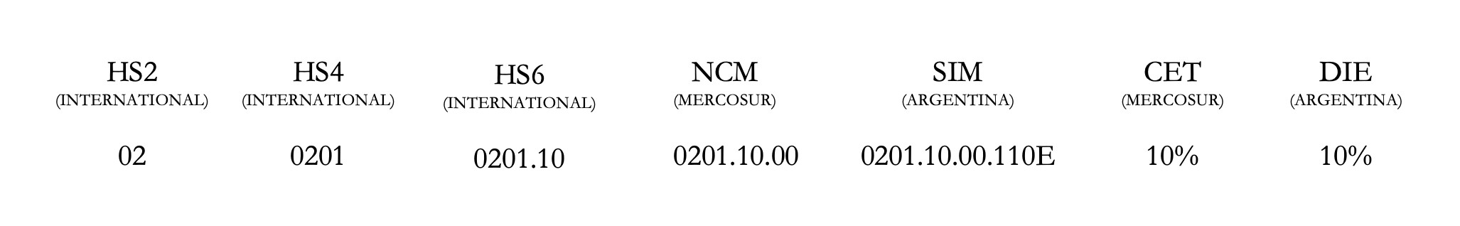
Tariff dispersion is not harmful in itself. We do not discuss the advantages and disadvantages of a flat import structure tariff or give policy recommendations in terms of the optimal import tariff. Instead, we focused on those cases in which tariff dispersion is unnecessary. For example, when ‘similar products’ have different import tariffs. Table 1 shows how two products from even two different HS2 codes are similar but have different import tariffs. When talking about Argentina’s import tariff structure, we talk about Derecho Importación Extrazona (DIE; Extra zone Import Duty), which, in general, is the same as the one defined by El Mercado Común del Sur (MERCOSUR, Southern Common Market), but it might differ in some specific cases. Table 2 is an example of two ‘similar products’ with the same HS2 but different HS4 and import tariffs. Table 3 is an example of two ‘similar products’ with even the same HS2, HS4, and HS6 (they only differ in terms of NCM)^[3] but with different import tariffs.

To answer whether tariff dispersion incentivises the red line in customs clearance, we exploited a full detailed dataset with information about Argentina’s imports from 2015–2018 and lane classification. We used the data to run a model with fixed effects. The data allowed us to control for importer, origin, product, custom and other non-tariff barriers.

We chose Argentina for two reasons, the first being data availability. We did not have any other data with this set of variables. Second, Argentina’s import structure tariff was adopted in the 1990s when MERCOSUR was created. When Argentina, Brazil, Uruguay and Paraguay decided to create a customs union, they also agreed on the Common External Tariff (CET). The import tariffs were defined following specific criteria of regional production. Those products with regional production would receive a high import tariff (relatively low for inputs and high for final goods), while those with no regional production would receive a 2 per cent import tariff. This allows us to believe that the tariff dispersion is not correlated to any other variable that might be correlated with customs clearance, allowing us to claim causality in our estimations.

This article builds on and aims to contribute to several strands of literature. First, to the best of our knowledge, it is the first paper that relates lane classification in Customs with import tariff dispersion. On the one hand, customs clearance and red lines have been discussed with a focus on administrative and legal purposes (Colagiovanni, 2020; Kuncoro et al., 2007). On the other, tariff dispersion has only been discussed or addressed in terms of trade negotiations (Cooper, 1964), trade discrimination (Becuwe & Blancheton, 2014; Ozerturk & Saggi, 2005), or revenues (Felbermayr et al., 2013; Fisman & Wei, 2004). Therefore, no link has been made previously between customs delays, red lines and tariff dispersion. Second, this article contributes to the discussion on optimal import tariff structures (Corden, 1976; Tarr, 2000) and adds a new argument in favour of simple import tariff structures.

This article is organised as follows. Section 2 briefly describes the customs clearance process in Argentina and the import tariff structure. Section 3 describes the data used in this paper and its limitations. Section 4 details the methodology while Section 5 summarises the results, and some robustness checks are performed. We conclude with Section 6.

2. Customs clearance and tariff dispersion

2.1. Customs clearance and the red lane

Every shipment at the customs border in Argentina is classified into a lane that might be green, orange, or red (Colagiovanni, 2020):

• Green Lane: The shipment is released since all the documentation complies with the legal requirements.

• Orange Lane: Additional checks must be done to decide if the shipment can enter the country; this does not imply merchandise control and verification.

• Red Lane: The shipment includes dangerous or hazardous materials (factory waste, damaged quality, dangerous chemicals, guns, etc.), or the paperwork seems incorrect. Physical inspection must be carried out.

It is important to note that the lane applies to every product in a shipment. In other words, a shipment can be composed of different products, and perhaps only one of these activates the red lane. For example, suppose there is a shipment composed of toys and chemicals. The toys may comply with all the legal requirements, but the chemicals must be controlled and checked, and the shipment goes to the red lane. In this case, the statistics would say that both the toys and the chemicals went through the red lane, even when toys would have been classified through the green lane if they were imported separately. This implies that we should only use single-product shipments (homogeneous shipments) in our analysis.

According to the literature, several factors are considered when classifying shipments into different lanes (Martincus et al., 2015; Ritzen-Pennings, 2020; Tanaka, 2011). In some cases, countries use risk management matrices to define the lane. In Argentina, according to recent literature (Colagiovanni, 2020), the following variables are considered for each product code:

• Non-Tariff Barriers (NTBs): HS codes with non-automatic licences (NALs), TBTs and PSMs are typically classified under orange or red lanes.

• Anti-Dumping Measures (ADMs): HS codes with antidumping measures — or undergoing investigations — are typically classified in the red lane.

• First Import: firms importing for the first time are automatically sent to the red lane.

• Import Reference Values (IRVs): some products have what is called IRVs, in other words, some products have an ‘official price’ as a reference. If this is the case, then the red lane is applied.

Even when some variables are publicly known as key determinants of the red lane, in many cases, it is not clear what criteria was used. In fact, if we consider the period 2015–2018, the share of imports going through the red lane changed substantially. In 2015, 43 per cent of the imports went to the red lane, while in 2018, this dropped to 22 per cent. This suggests that other variables, not explicit in any regulation or law, might be affecting the probability of a red lane for any one shipment. We used a wide set of controls such as origin, customs, year, chapter (HS2), and interaction between customs and chapter, to account for these other variables.

Lastly, misclassification also leads to the red lane. If it is believed the importer is trying to import a product under the wrong code, then physical inspection (red lane) is required. Getting the right classification is not only important in its own right but also because of tax revenues. This problem does not exist if the import tariff structure is flat and increases when tariff dispersion is high.

2.2. Tariff dispersion

In this paper, we focus on Argentina’s import tariff structure and its dispersion. As previously stated, Argentina relies on the HS classification until the 6-digit level (HS6) but adds two additional levels: NCM (8-digit level) and Sistema Informático Malvina (SIM; Malvina Computer System) (12-digit level).

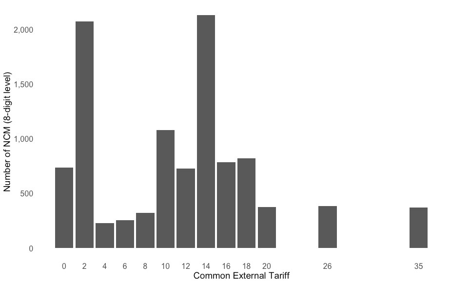
MERCOSUR’s tariff structure, CET — and, therefore, Argentina’s tariff structure — was defined in the 1990s. It is a long way from being a flat tariff, and it is usually higher for final goods. The import tariff is defined at the NCM level. Those products with no regional production have an import tariff of 2 per cent. However, even though the four countries agreed on the idea of a CET, many exceptions apply in practice, with both external deviations from the CET and internal deviations from free trade. Figure 1 shows a specific product (meat) as an example of the HS codes (2-, 4- and 6-digit level), NCM (8-digit level), SIM (12-digit level) and the CET and DIE. Figure 2 shows CET’s distribution. As previously noted, there are a lot of products (20%) where the import tariff equals 2 per cent.

Figure 1.Common External Tariff

Source: Authors, based on Ministry of Economics of the Republic of Argentina (n.d.)

Figure 2.Common External Tariff 2019

Source: Authors, based on Ministry of Economics of the Republic of Argentina (n.d.)

When two products share the same HS4 code but have different import tariffs at the 6-digit level, we talk about tariff dispersion at the HS4 level. When they share the same HS6 level but have different import tariffs at the NCM level, we talk about tariff dispersion at the HS6 level. Lastly, when the products belong to the same NCM but have different import tariffs at the SIM level, we talk about tariff dispersion at the NCM level.

We mainly focus on the tariff dispersion at the HS6 level, like the one shown in Table 3. Formally, the tariff dispersion is a binary variable, D_pt, defined as:

$$\small D_{pt}= \begin{cases}1, & \text { if subheading }(\mathrm{HS} 6) \text { of product } p \text { being imported in year } t \\ & \text { has more than one tariff line at the } 8 \text {-digit level, } \\ 0, & \text { if otherwise. }\end{cases}\tag{1}$$

More tariff dispersion is expected at the HS4 level than at the NCM level. This is because even when they belong to the same HS4 code, products might still be very different. On the contrary, products belonging to the same NCM are more likely to be similar, and they will also have the same CET since the CET was defined at the NCM level. Therefore, to have tariff dispersion at the NCM level, Argentina’s government must be deviating from the CET using one of the allowed mechanisms.

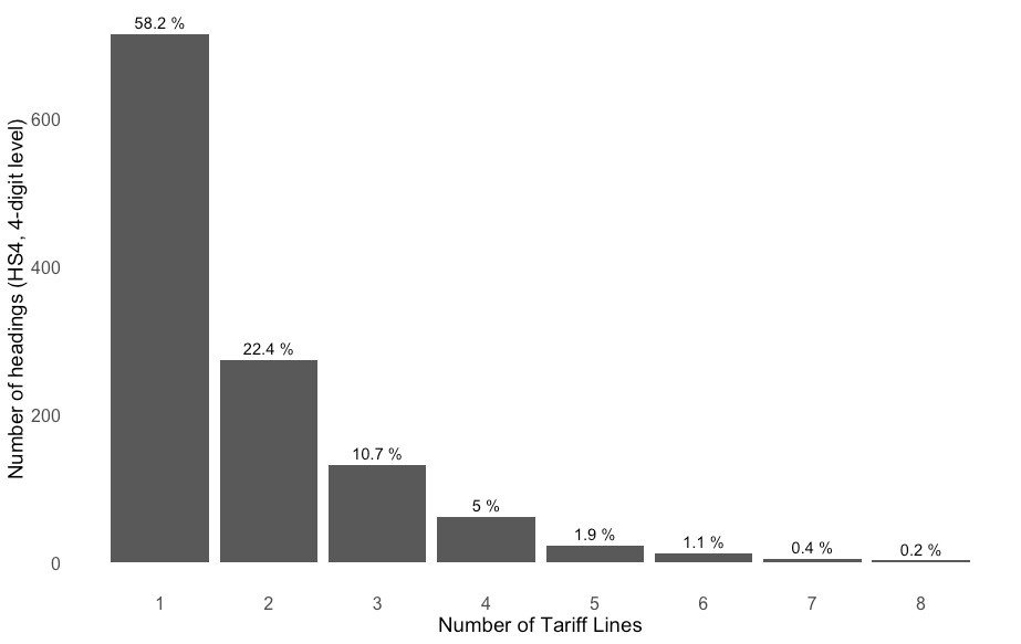
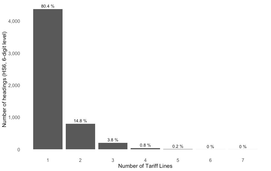
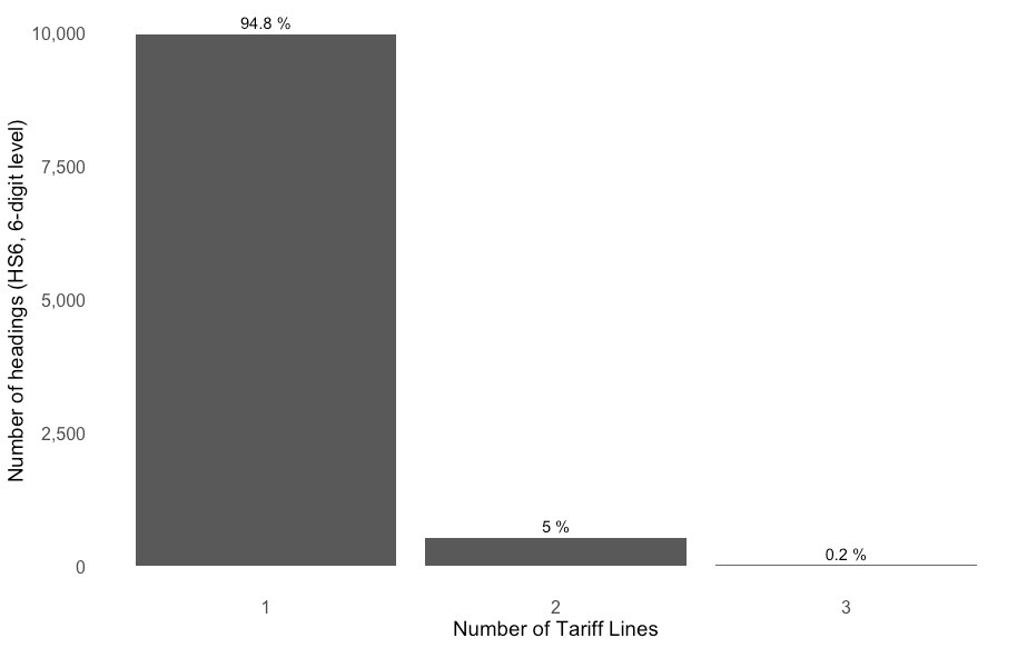
Our analysis covers 2015 to 2018. The dataset is only available for those years and periods, and therefore, data availability is the only restriction guiding our analysis. In 2015, 58.2 per cent of the headings (HS4) had only one tariff line — that is, no tariff dispersion — as shown in Figure 3. At the HS6 level, tariff dispersion is lower but still high: around 20 per cent of the subheadings have more than one tariff line (Figure 4). As expected, tariff dispersion is very low at the NCM level (Figure 5). The three figures show us that as we change the definition of tariff dispersion (Equation (1)), the number of products belonging to a heading, subheading or NCM with tariff dispersion changes significantly: 41.8 per cent of the headings have more than one tariff line, while this number is 19.6 per cent for the subheadings and just 5.2 per cent for the NCM.

Figure 3.Tariff dispersion at the HS4 level — DIE

Source: Authors, based on Ministry of Economics of the Republic of Argentina (n.d.)

Figure 4.Tariff dispersion at the HS6 level 0151 — DIE

Source: Authors, based on Ministry of Economics of the Republic of Argentina (n.d.)

Figure 5.Tariff dispersion at the NCM level — DIE

Source: Authors, based on Ministry of Economics of the Republic of Argentina (n.d.)

We wanted to know if products belonging to headings (4-digit), subheadings (6-digit), or NCMs (8-digit) with tariff dispersion are more likely to be classified through the red line.

3. Data

To address this question, we used data for Argentina’s 2015–2018 imports obtained from the Dirección General de Aduanas (DGA, General Directorate of Customs). This is our core dataset. It contained information about the product (at the 12-digit level), origin, price, quantity, lane, importer, and date for every import made during those four years. This information was obtained from the Ministry of Production in Argentina.

We also constructed original datasets related to relevant commercial policies. We tracked every policy related to ADMs and IRVs measures, and NAL changes. For anti-dumping, we used information obtained from VUCE. For IRV, we used information from Administración Federal de Ingresos Públicos (AFIP), Argentina’s Revenue Agency, and considered Resolution 2730/09 and its modifications. For Non-Automatic Licensing (NLA), we tracked measures 5/15 – E 292/17, 2/16 – 32/16 – 114/16 – 264/16 – E 301/16 – E 152/17 – E 523/17 – E 898/17 – E 5/18 170/18 – 507/18 – 526/18. Every measure was read and analysed using the website Information Legislativa y Documental (InfoLEG), an online portal with information about every law and measure published by the government (Argentina National Congress, n.d.). All this information is publicly available.

Lastly, we also added controls using the importer’s size, measured by the number of employees, obtained from AFIP. Table 4 describes each variable.

Since we had information at the product level, we knew if the product was subject to other measures, such as anti-dumping or NTBs like import licensing systems. We created different datasets to merge them into the one obtained from the DGA following findings from Colagiovanni (2020) on which variables are used the most frequently in Argentinian Customs to classify shipments into the three lanes, such as IRVs, AMDs, NTBs such as NALs, TBT and PSM.

As previously mentioned, we needed to keep only those shipments with a single product, which we called ‘homogeneous’ shipments. If there was more than one HS code in a shipment, we could not determine which product generated the red lane.

4. Methodology

To estimate if ‘similar products’ with different tariffs are, on average, more likely to be classified through the red lane, we used the following regression:

$$Y_{ipoct}=\beta_1 D_{pt}+\delta X_{ipoct}+\gamma_t+\eta_p+\lambda_{i, o, c}+\zeta_{c p}+\varepsilon_{ipoct} \tag{2}$$

where Y_ipoct is a dummy that takes a value of 1 if import of firm i and product p from origin o and custom office c in year t was assigned to the red lane and 0 otherwise; D_pt is a dummy that takes a value of 1 if the product p being imported in year t belongs to a sub-heading (HS6) with tariff dispersion and 0 otherwise. The variable X_ipoct is a set of control variables related to each importer i, product p, origin o, custom office c in year t (mainly variables strongly correlated with the probability of being classified in a red lane). γ_t and η_p are year and product (chapter — HS2 level) fixed effects. λ_i,o,c are fixed effects by importer i, origin o and customs office c. ζ_cp is the interaction between product (chapter) and customs office c, and also works as a fixed effect. ε_ipoct is the error term, and we used cluster standard errors at the firm level (Bertrand et al., 2004).

Another important aspect is how we generated D_pt. In our main regression, we used the CET import tariff structure. That is, we considered all the codes. In the robustness check subsection, we generated D_pt considering only those codes where there were imports in Argentina during the period 2012–2019^[4] and then during the period 2015–2018 in only homogeneous shipments.

Our main interest was on β₁. This parameter answered our question about the link between tariff dispersion and the red lane. It could be said that because tariff dispersion is not randomly generated, we were not capturing a causal effect. Even though it is true that the import tariff structure is not randomly defined, we argue that the tariff dispersion at the HS6 level is generated by reasons not correlated with any variable in the error term. In most cases, tariff dispersion appeared when some products had an import tariff of 2 per cent. The general rule in MERCOSUR is to assign a 2 per cent import tariff to those products without regional production. In other words, products have an import tariff higher than 2 per cent if they are produced by one or more countries and 2 per cent otherwise. Therefore, we generated D_pt at the HS6 level, like in the example in Table 3. This allowed us to strengthen our methodology and identification strategy. Since tariff dispersion was mostly generated by exogenous reasons related to regional production criteria, and since we added fixed controls by year, origin, customs, chapter HS, importer, and the interaction chapter and origin, we believe that β₁ captured a causal effect. In other words, it is tariff dispersion that increased the red lane classification.

In the robustness check subsection, we ran the model generating D_pt at the HS4 and NCM levels. Selection bias was more likely in the latter. This is because when looking at tariff dispersion at the NCM level, we were looking for those NCMs with different tariff lines at the SIM level. If this is the case, it is because Argentina changed the import tariff, and this is done in very specific cases, mostly related to protectionism, which might correlate with tougher inspections at Customs and higher barriers to import.

5. Results

5.1. Regression results

Table 5 summarises the main findings from Equation 1. As expected, new importers, products with anti-dumping investigations or current measures, IRVs, or NTBs such as NAL were more likely to be classified into the red lane. More importantly, our coefficient of interest, the tariff dispersion, was positive, significant and stable over different regressions with different controls. In other words, products belonging to subheadings with more than one tariff level were more likely to be classified into the red lane. The coefficient was high, 2.9 percentage points, implying that products associated with tariff dispersion were 10 per cent more likely to be classified in the red lane.

In addition, Table 6 shows that the effect was larger when the tariff heterogeneity was high (i.e., the difference between the tariff levels was high, and higher than 12 percentage points). The results held for the definition of tariff dispersion at the 4-digit level (column 1) and the 6-digit level (column 3), but not at the 8-digit level (expected positive (+) effect with high dispersion but not statistically significant), but it makes sense since having tariff dispersion at the 8-digit level is not common (Figure 5), since it requires a specific and unilateral change of the import tariff by Argentina. In other words, in the first column, Equation (1) takes the value 1 when a SIM code belongs to a HS4 with more than one duty level, while in the second column Equation (1) takes value 1 when the product code at the SIM level belongs to a HS6 with more than one duty level, and lastly, the third column takes value 1 in Equation (1) when the product belongs to a NCM with more than one duty level.

5.2. Robustness check

In this subsection, we ran the model using different definitions of tariff dispersion and for all the tariff dispersion levels. In our calculations, we considered all the HS codes. In this section, we modify the dataset to see if the results held.

First, we considered only those HS codes with imports higher than 0 during the period 2012 to 2019. Our argument says that when you have two NCMs with the same HS6 but a different import tariff, then the red lane might be more likely due to the need to get the right classification for the product being imported. In the previous section, we defined tariff dispersion following Equation (1) using every NCM and its import tariff. Now, we define tariff dispersion following the same equation but dropping those NCMs that were never used. If an NCM is never used to classify a product, then the red lane is more unlikely: no matter the tariff dispersion, it is unlikely that a product could be classified using an NCM that was never used. The results are shown in Table 7, in columns (2), (4), and (6). We did not see significant changes in β₁ between column (3) — the original estimation at the HS6 level — and column (4).

Conclusion

Even though delays in Customs have been widely studied in terms of their impacts, there is little evidence concerning their cause(s). This paper addresses a new hypothesis. In some cases, it might be the complex and dispersed import tariff structure that creates unnecessary delays through physical inspection at customs.

We exploited a detailed and original dataset with information about Argentina’s imports between 2015 and 2018 and the fact that in MERCOSUR, most tariff dispersion was generated due to ‘regional production’ criteria to run a model with fixed effects and estimate the link between tariff dispersion and the red lane in customs clearance. In other words, some products have a 2 per cent import tariff because there is no regional production in MERCOSUR, while another product in the same subheading might have 12 per cent. Since the tariff difference, and therefore tariff dispersion, was generated by this ‘regional production’ criteria, we can estimate the link.

Our results showed that products that might be classified into two different codes with different import tariffs were more likely to be classified through the red lane. We also found that new importers and products with either ADMs, NAL, or IRVs were also more likely to go through the red lane, as predicted.

We found that shipments of products belonging to an HS6 with tariff dispersion at the 8-digit level (NCM dispersion) were 2.9 percentage points more likely to be sent to the red lane. When the import tariff difference was low, the effect disappeared; when it was high, the number increased to 5.0 percentage points. Considering that around 40 per cent of imports are sent to the red lane, this implies that high levels of tariff dispersion are associated with a 10 per cent increase in the probability of being classified in the red lane.

These results have important implications. Having an import tariff structure with high levels of tariff dispersion might add unnecessary costs to imports in terms of time and money. Considering the advantages of a fast and efficient Customs (Marti et al., 2014; Martincus et al., 2013; Sanchez et al., 2003), simplification of the tariff import structure to avoid unnecessary tariff dispersion is recommended. The red lane should be used for essential verification and controls (those related to quality standards or hazardous materials or drugs, for example), not to discuss product classifications.

These results highlight a new, different and positive side to having a simple and homogeneous import tariff structure. When ‘similar products’ have different import tariffs, misclassification, or problems at Customs might arise, generating unnecessary delays.

If a flat import tariff structure is not feasible, then countries must ensure they do not have tariff dispersion at high levels of the HS code. In other words, even though different headings (HS4) may have different import tariffs due to industrial policy goals or specific tariff protection for some products, it is important to have low tariff dispersion when comparing subheadings (HS6) of the same headings (HS4).